1 package

Code

library(tidyverse)
library(ggplot2)
library(tidymodels)
library(rsample)
library(themis)
library(tidytuesdayR)

library(scales)
library(lubridate)

library(anytime)

2 data

download data from https://chip-dataset.vercel.app/

Code

raw_chips <- read_csv("data/chip_dataset.csv")

Code

chips <- raw_chips %>%
  select(-1) %>%
  janitor::clean_names() %>%
  mutate(old_release_date=release_date
         ,process_size_nm=as.numeric(process_size_nm)
          ,release_date_pre = as.Date(release_date, format = "%m/%d/%Y")
         ,transistors_million=as.numeric(transistors_million)
         ,transistors = transistors_million * 1000000
         ,year = year(release_date_pre)+2000
         ,month=month(release_date_pre)
         ,day=day(release_date_pre)
         ,release_date=make_date(year,month,day)
         ) %>% filter(year<=2023)

Code

head(chips)

# A tibble: 6 × 18
  type  release_date process_size_nm tdp_w die_size_mm_2 transistors_million
  <chr> <date>                 <dbl> <chr> <chr>                       <dbl>
1 CPU   2000-06-05               180 54    120                            37
2 CPU   2000-10-31               180 54    120                            37
3 CPU   2000-08-14               180 60    120                            37
4 CPU   2000-10-31               180 63    120                            37
5 CPU   2000-10-31               180 66    120                            37
6 CPU   2000-10-17               180 66    120                            37
# ℹ 12 more variables: freq_g_hz <dbl>, foundry <chr>, vendor <chr>,
#   fp16_gflops <dbl>, fp32_gflops <dbl>, fp64_gflops <dbl>,
#   old_release_date <chr>, release_date_pre <date>, transistors <dbl>,
#   year <dbl>, month <dbl>, day <int>

Code

dim(chips)

[1] 4707   18

2.1 EDA

Code

chips %>%
  count(type)

# A tibble: 2 × 2
  type      n
  <chr> <int>
1 CPU    2148
2 GPU    2559

Code

chips %>%
  count(year = year(release_date),
        type) %>%
  ggplot(aes(year, n, fill = type)) +
  geom_col() +
  labs(x = "Year",
       y = "# of chips")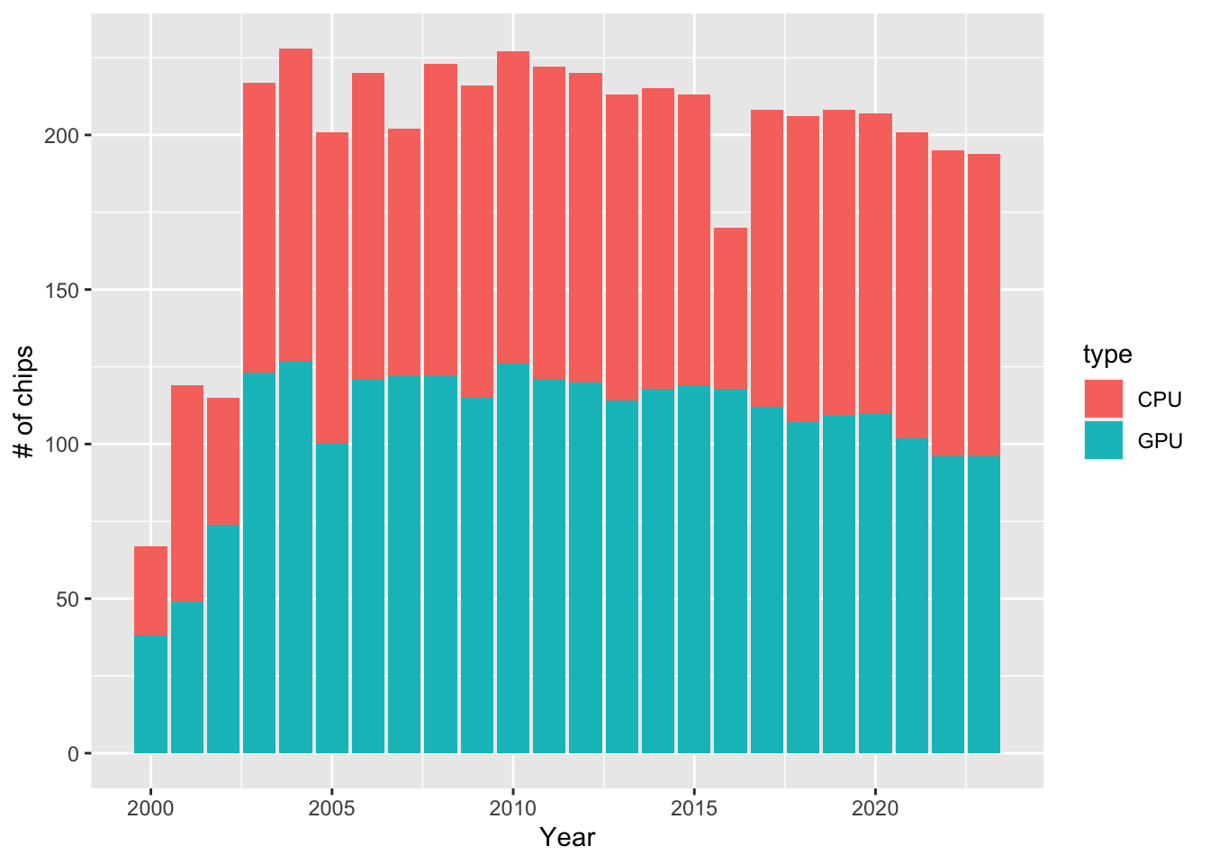

Code

chips %>%
  ggplot(aes(transistors_million)) +
  geom_histogram() +
  scale_x_log10(labels = label_number(suffix = "M", big.mark = ","))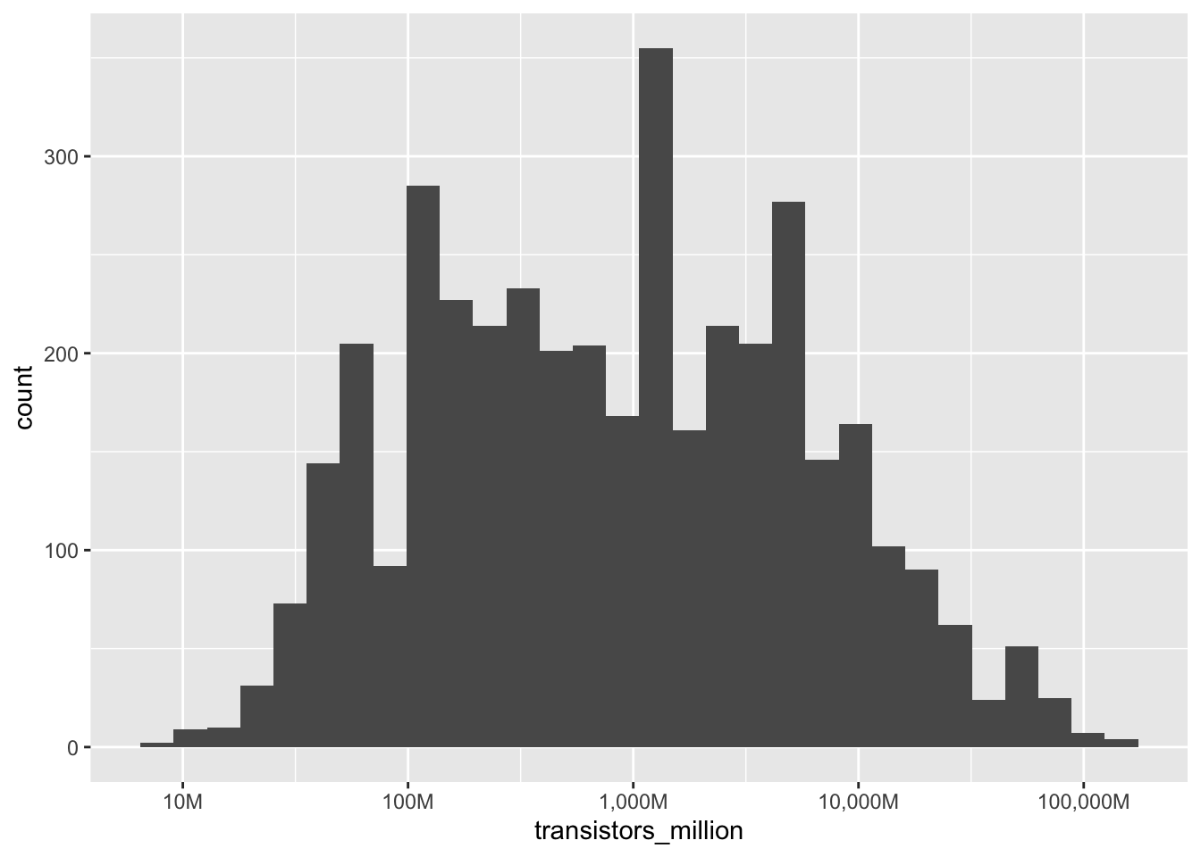

Code

summarize_chips <- function(tbl) {
  tbl %>%
    summarize(pct_gpu = mean(type == "GPU"),
              median_transistors = median(transistors, na.rm = TRUE),
              geom_mean_transistors = exp(mean(log(transistors), na.rm = TRUE)),
              n = n(),
              .groups = "drop") %>%
    arrange(desc(n))
}

Code

chips %>%
  group_by(year = year(release_date)) %>%
  summarize_chips() %>%
  ggplot(aes(year, median_transistors)) +
  geom_line()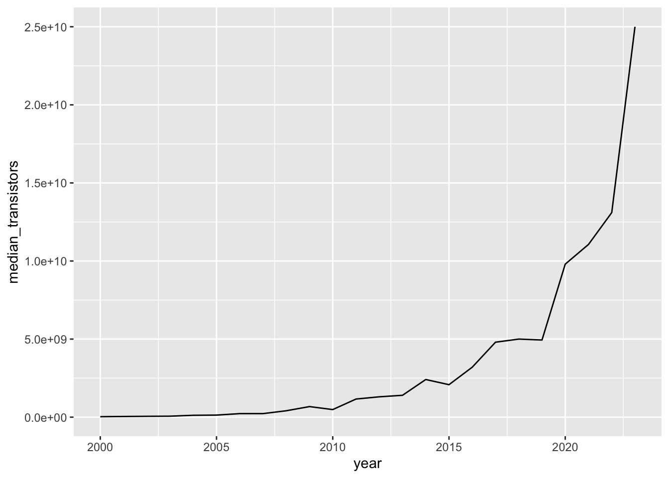

Code

chips %>%
  mutate(years_since_2000 = as.integer(release_date - as.Date("2000-01-01")) / 365) %>%
  mutate(moores_law = 30 * 2 ^ (.5 * years_since_2000)) %>%
  ggplot(aes(release_date, transistors_million)) +
  geom_point() +
  geom_line(aes(y = moores_law), color = "red") +
  geom_smooth(method = "loess") +
  scale_y_log10() +
  labs(x = "Chip release date",
       y = "# of transistors (millions)",
       title = "We are a bit below Moore's Law")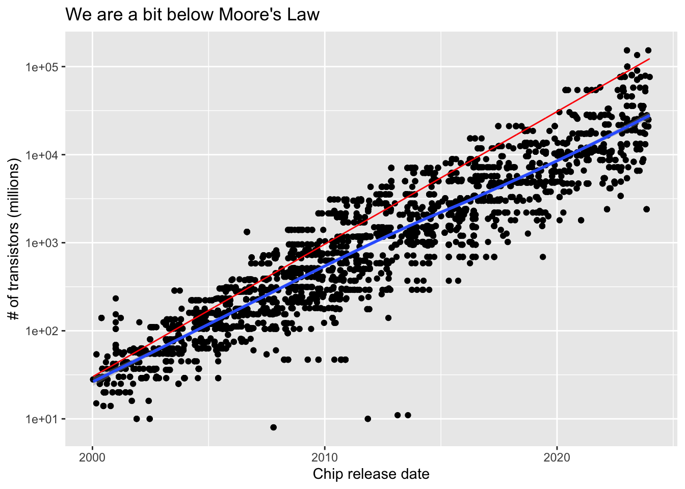

Code

chips %>%
  group_by(foundry = fct_lump(foundry, 6),
           type) %>%
  summarize_chips() %>%
  mutate(foundry = fct_reorder(foundry, n, sum)) %>%
  ggplot(aes(n, foundry, fill = type)) +
  geom_col() +
  labs(y = "Chip creator")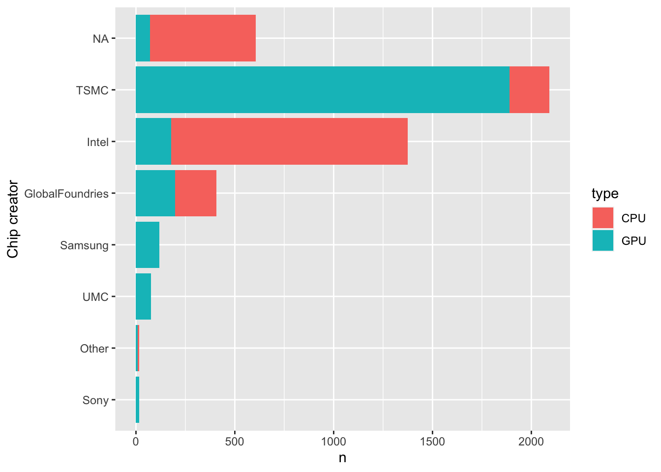

Code

chips %>%
  group_by(foundry = fct_lump(foundry, 2),
           year) %>%
  summarize_chips() %>%
  ggplot(aes(year, median_transistors, color = foundry)) +
  geom_line() +
  scale_y_log10()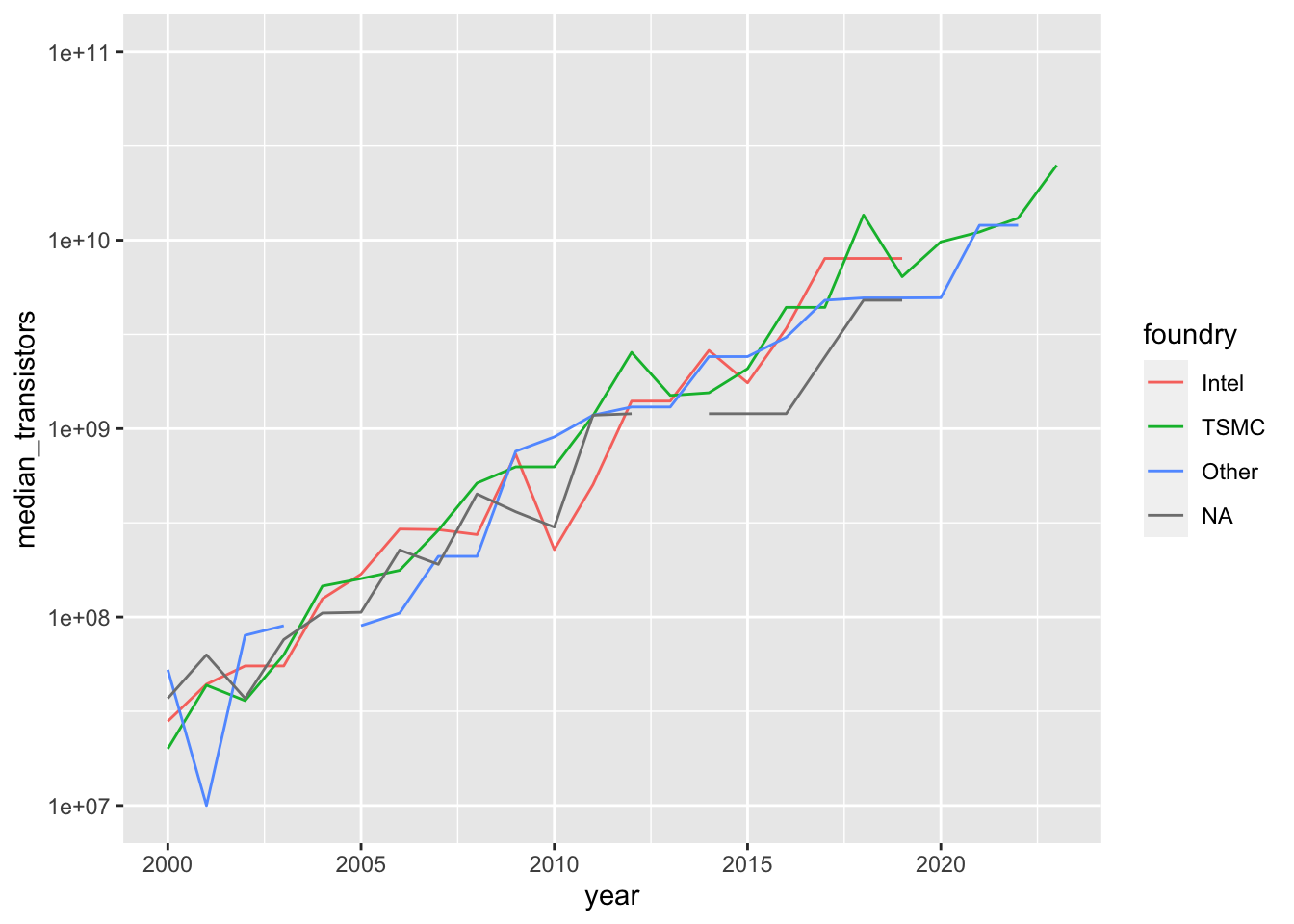

Code

chips %>%
  mutate(foundry = fct_lump(foundry, 2)) %>%
  ggplot(aes(release_date, transistors_million,
             color = foundry)) +
  geom_point(alpha = .1) +
  geom_smooth(method = "lm") +
  scale_y_log10() +
  labs(x = "Chip release date",
       y = "# of transistors (millions)")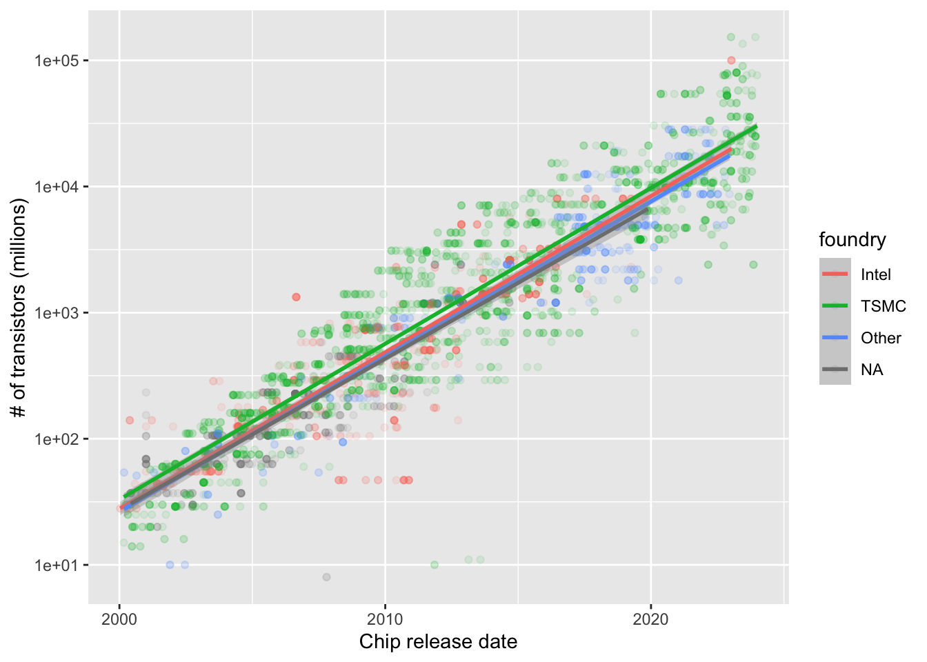

Code

chips %>%
  ggplot(aes(fp64_gflops)) +
  geom_histogram() +
  scale_x_log10()

Code

chips %>%
  filter(!is.na(fp32_gflops)) %>%
  ggplot(aes(release_date,
             fp32_gflops)) +
  geom_point() +
  geom_smooth(method = "lm") +
  scale_y_log10() +
  labs(x = "Chip release date",
       y = "Gigaflops (fp64)")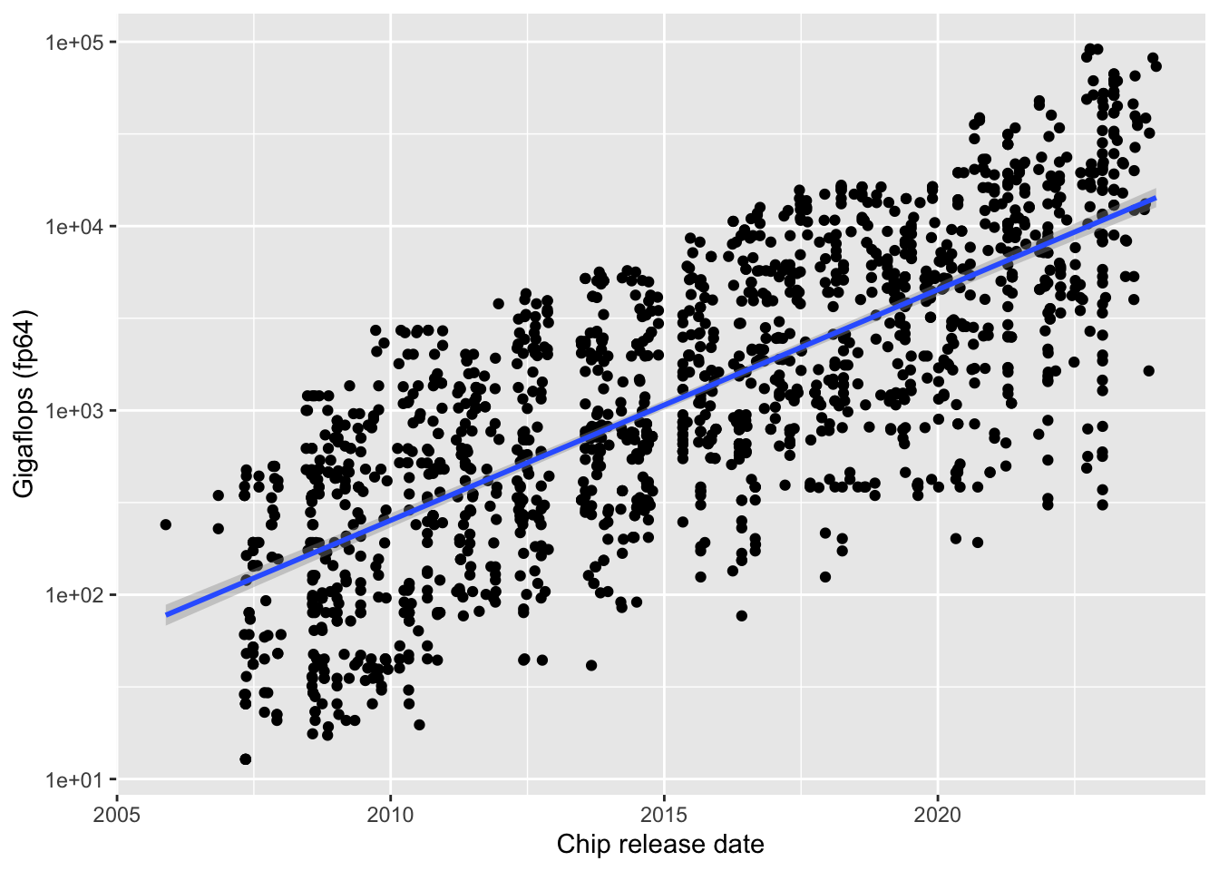

Code

chips %>%
  filter(!is.na(fp32_gflops)) %>%
  group_by(year) %>%
  filter(n() >= 50) %>%
  ggplot(aes(transistors_million, fp32_gflops)) +
  geom_point() +
  facet_wrap(~ year, scales = "free") +
  scale_x_log10() +
  scale_y_log10()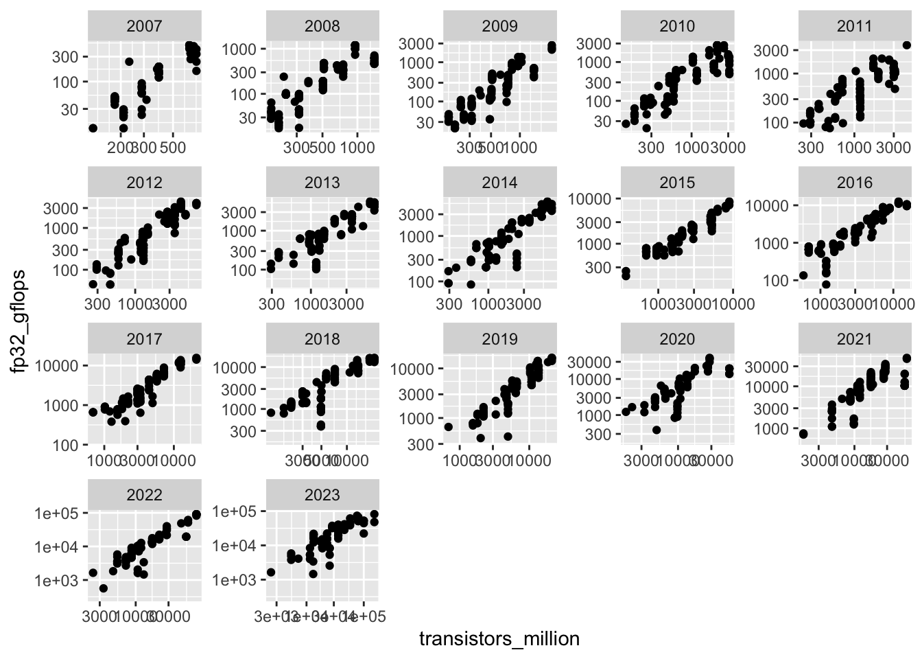

Code

chips %>%
  ggplot(aes(release_date, process_size_nm)) +
  geom_point() +
  scale_y_log10()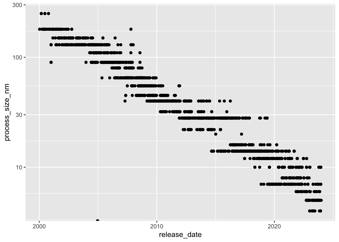

Code

lm(log(fp64_gflops) ~
     log(transistors), data = chips) %>%
  summary()


Call:
lm(formula = log(fp64_gflops) ~ log(transistors), data = chips)

Residuals:
    Min      1Q  Median      3Q     Max 
-2.1678 -0.6779 -0.1022  0.4162  3.0476 

Coefficients:
                  Estimate Std. Error t value Pr(>|t|)    
(Intercept)      -17.76561    0.53241  -33.37   <2e-16 ***
log(transistors)   1.02853    0.02395   42.95   <2e-16 ***
---
Signif. codes:  0 '***' 0.001 '**' 0.01 '*' 0.05 '.' 0.1 ' ' 1

Residual standard error: 0.971 on 1113 degrees of freedom
  (3592 observations deleted due to missingness)
Multiple R-squared:  0.6237,    Adjusted R-squared:  0.6234 
F-statistic:  1845 on 1 and 1113 DF,  p-value: < 2.2e-16

3 Reference

https://www.youtube.com/watch?v=EPusvEQuO2A

https://github.com/rfordatascience/tidytuesday/tree/master/data/2022/2022-08-23

https://github.com/dgrtwo/data-screencasts/blob/master/2022_08_23_chips.Rmd